Triple Well Spatio-temporal Decorrelation
import numpy as np
import pyemma.msm as msm
import msmtools.generation as msmgen
import msmtools.analysis as msmana
import pyemma.coordinates as coor
import matplotlib.pylab as plt
import anca
%pylab inline
plt.style.use('ggplot')
Populating the interactive namespace from numpy and matplotlib
/Users/fxp/anaconda2/lib/python2.7/site-packages/IPython/core/magics/pylab.py:161: UserWarning: pylab import has clobbered these variables: ['plt']
%matplotlib prevents importing * from pylab and numpy
  "n`%matplotlib` prevents importing * from pylab and numpy"
def assign(X, cc):
    T = X.shape[0]
    I = np.zeros((T),dtype=int)
    for t in range(T):
        dists = X[t] - cc
        dists = dists ** 2
        I[t] = np.argmin(dists)
    return I
P = np.array([[0.75, 0.05, 0.2],
[0.05, 0.75, 0.2],
[0.2, 0.05, 0.75]]);
T = 100000
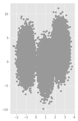
means = [np.array([-1,1]), np.array([1,-1]), np.array([2.5,2.5])];
widths = [np.array([0.3,2]),np.array([0.3,2]), np.array([0.3,2])];
# continuous trajectory
X = np.zeros((T, 2))
# hidden trajectory
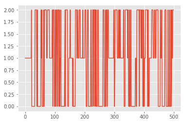
dtraj = msmgen.generate_traj(P, T)
for t in range(T):
s = dtraj[t]
X[t,0] = widths[s][0] * numpy.random.randn() + means[s][0]
X[t,1] = widths[s][1] * numpy.random.randn() + means[s][1]
dtraj.shape
(100000,)
plt.plot(dtraj[0:500]);
plt.figure(figsize=(4,7))
plt.scatter(X[:,0], X[:,1], marker = 'o', color=[0.6,0.6,0.6])
<matplotlib.collections.PathCollection at 0x111ef6690>
Spatial Decorrelation of Order 2 (SD2)
Parameters:
data – a 3n x T data matrix (number 3 is due to the x,y,z coordinates for each atom). Maybe a numpy
array or a matrix where,

n: size of the protein

T: number of snapshots of MD trajectory

m: dimensionality of the subspace we are interested in; Default value is None, in which case m = n

verbose: print information on progress. Default is true.
Returns:
A 3n x m matrix U (NumPy matrix type), such that Y = U * data is a 2nd order spatially whitened
coordinates extracted from the 3n x T data matrix. If m is omitted, U is a square 3n x 3n matrix.

Ds: has eigen values sorted by increasing variance

PCs: holds the index for m most significant principal components by decreasing variance S = Ds[PCs]

S – Eigen values of the ‘data’ covariance matrix

B – Eigen vectors of the ‘data’ covariance matrix. The eigen vectors are orthogonal.
from pyANCA import SD2
(Y, S, B, U) = SD2.SD2(X, m=2);
2nd order Spatial Decorrelation -> Looking for 2 sources
2nd order Spatial Decorrelation -> Removing the mean value
2nd order Spatial Decorrelation -> Whitening the data
Temporal Decorrelation of Order 2 (TD2)
Parameters:
Y -- an mxT spatially whitened matrix (m dimensionality of subspace, T snapshots).
May be a numpy array or a matrix where,

m -- dimensionality of the subspace we are interested in. Defaults to None, in which case m=n.
T -- number of snapshots of MD trajectory

U -- whitening matrix obtained after doing the PCA analysis on m components of real data

lag -- lag time in the form of an integer denoting the time steps

verbose -- print info on progress. Default is True.
Returns:
V -- An n x m matrix V (NumPy matrix type) is a separating matrix such that V = Btd2 x U
(U is obtained from SD2 of data matrix and Btd2 is obtained from time-delayed covariance of matrix Y)

Z -- Z = B2td2 * Y is spatially whitened and temporally decorrelated (2nd order) source extracted from
the m x T spatially whitened matrix Y.

Dstd2: has eigen values sorted by increasing variance

PCstd2: holds the index for m most significant principal components by decreasing variance
R = Dstd2[PCstd2]

R – Eigen values of the time-delayed covariance matrix of Y

Btd2 – Eigen vectors of the time-delayed covariance matrix of Y
from pyANCA import TD2
(Z, R, Btd2, V) = TD2.TD2(Y, m=2, U=U, lag=5)
2nd order Temporal Decorrelation -> Looking for 2 sources
2nd order Temporal Decorrelation -> Removing the mean value
2nd order Temporal Decorrelation -> Whitening the data
Temporal Decorrelation of Order 4 (TD4)
Parameters:
Z -- an mxT spatially uncorrelated of order 2 and temporally uncorrelated of order 2 matrix (m subspaces, T
samples). May be a numpyarray or matrix where

m - number of subspaces we are interested in.
T - Number of snapshots of MD trajectory

V -- separating matrix obtained after doing the PCA analysis on m
components of real data followed temporal decorrelation of the spatially whitened data

lag -- lag time in the form of an integer denoting the time steps

verbose -- print info on progress. Default is True.
Returns:
W -- separating matrix
from pyANCA import TD4
W = TD4.TD4(Z, m=2, V=V, lag=5)
4th order Temporal Decorrelation -> Estimating cumulant matrices
TD4 -> Contrast optimization by joint diagonalization
TD4 -> Sweep #  0 completed in 1 rotations
TD4 -> Sweep #  1 completed in 0 rotations
TD4 -> Total of 1 Givens rotations
TD4 -> Sorting the components
TD4 -> Fixing the signs
(2, 2)
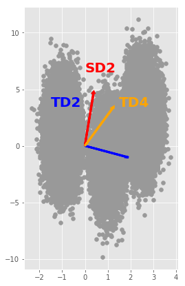
def draw_arrow(a, v, color):
    plt.arrow(0, 0, a*v[0], a*v[1], color=color, width=0.02, linewidth=3)
plt.figure(figsize=(4,7))
scatter(X[:,0], X[:,1], marker = 'o', color=[0.6,0.6,0.6])

plt.arrow(0, 0, 3*U[0,0], 12*U[0,1], color='red', width=0.02, linewidth=3);
plt.text(-0.0, 6.5, 'SD2', color='red', fontsize=20, fontweight='bold', rotation='horizontal')

plt.arrow(0, 0, 3*V[0,0], 4*V[0,1], color='blue', width=0.02, linewidth=3);
plt.text(-1.5, 3.5, 'TD2', color='blue', fontsize = 20, fontweight='bold', rotation='horizontal')

plt.arrow(0, 0, 7*W[0,0], 9*W[0,1], color='orange', width=0.02, linewidth=3);
plt.text(1.5, 3.5, 'TD4', color='orange', fontsize=20, fontweight='bold', rotation='horizontal')
<matplotlib.text.Text at 0x1131fb050>
YTD4 = W.dot(Z);
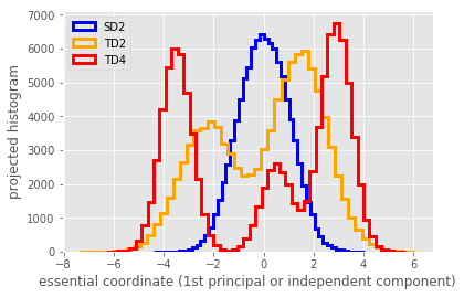
hist(Y[0,:].T, bins=50, histtype='step', linewidth=3, label='SD2', color='blue')
hist(0.5*Z[0,:].T, bins=50, histtype='step', linewidth=3, label='TD2', color='orange')
hist(YTD4[1,:].T, bins=50, histtype='step', linewidth=3, label='TD4', color='red')

xlabel('essential coordinate (1st principal or independent component)')
ylabel('projected histogram')
legend()
<matplotlib.legend.Legend at 0x111ebe550>